How to dock
flexible cyclic molecules with AutoDock and live happy
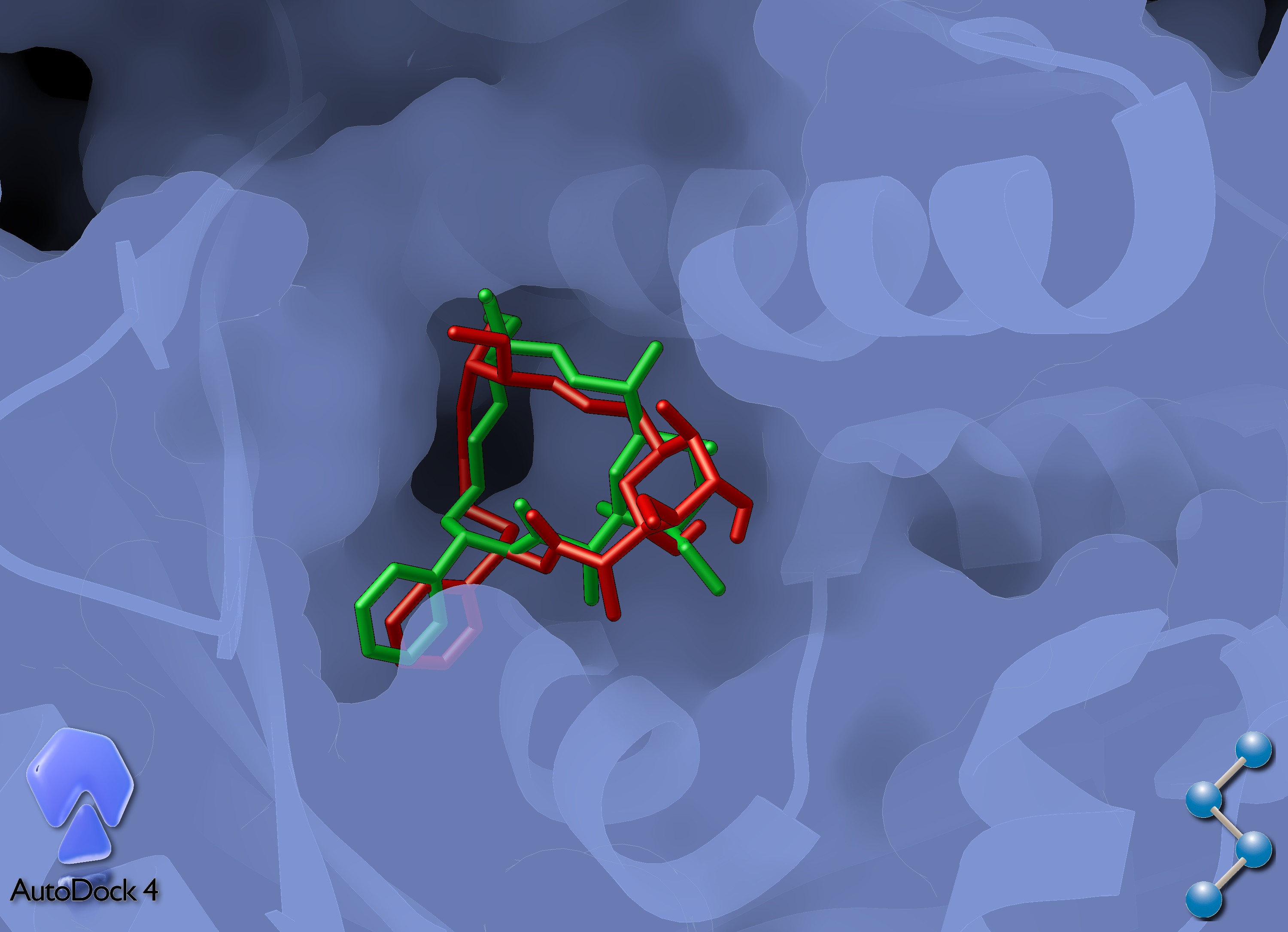
Soraphen-A antibiotic docked to the acetyl-coenzime A carboxylase (PDB id 1W96)
Introduction
AutoDock
is not able to manage directly
the flexibility associated to bonds comprised in cyclic molecules.
The genetic algorithm is indeed not able to modify rotatable bonds in
a concerted fashion, then the rotation of an intra-cyclic bond would
lead to a distorted structure. For this reason, cyclic portions of
the ligands are considered as rigid. Different approaches can be used
todock macrocyclic
molecules, usually identifying one
(or many) low energy conformations and dock them as different
ligand(s).
But
using an indirect method, is
possible to manage the ring as a fully flexible entity and use the
AutoDock GA to explore its flexibility. The method was initially
developed for
the version 3.05 [PubMed],
while now is officially
implemented since version 4.2.
The method
The
protocol consists basically in
converting the cyclic ligand into its corresponding acyclic form by
breaking a bond and dock it as fully flexible, letting AutoDock to
restore the original cycle structure during the calculation by means of
special (G, glue) atom types.
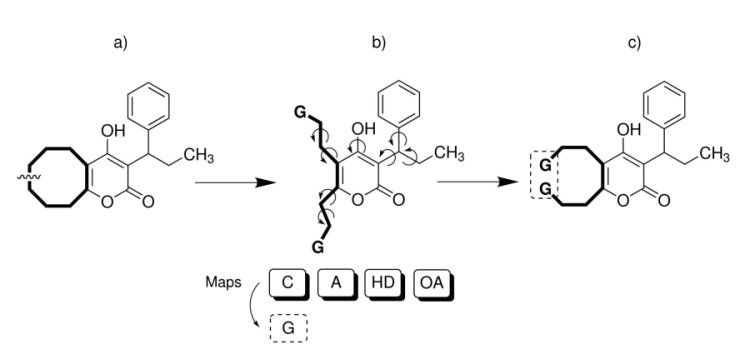
The protocol can be subdivided in three main steps:
Ring opening (a):
by
removing a bond, the ring is opened and the ligand is transformed to
an acyclic form.
Ligand pre-processing (b):
the
ligand is processed following the standard AutoDockTools protocol,
but the edge atoms are replaced with G atoms.
Docking and ring closure (c):
the
ligand is docked applying a 12-2 pseudo-Lennard-Jones potential to
the G-atoms that restore the cyclic structure (see the AutoDock User Guide for details).
Guidelines
To convert the molecule into the acyclic
form one bond to be broken must be identified. The way the acyclic form
is obtained can affect the calculation and the ring closure.
- The
following advices can be useful when choosing the breaking bond:
Keep number rotatable
bonds low
The ring opening can increase
dramatically
the total number of rotatable bonds, requiring longer calculation
times. Therefore, when less flexible or partially rigid regions are
present (i.e. conjugated bonds) they should not be broken. Any further
information available (i.e. NMR studies) should be used to keep
rotatable bonds fixed.
|
Break carbon-carbon
bonds
The atoms formerly connected by
the broken bond will be "transformed" into glue atoms, but they are actual
carbon atoms. This will allow to simplify the calculation setup by
using a single extra atom type and refer it to the actual C.map file.
|
Avoid chiral atoms
(...whenever possible)
If a bond between one or
more chiral carbon atoms is broken, original chirality is not guaranted in the resulting
closed ring. Often cyclic molecules present many chiral centers (i.e.
natural compounds, antibiotics) then identify bonds between achiral
carbons is not possible. In this case, any carbon-carbon bond can be
suitable, while chirality in docking results should be inspected and
manually corrected if needed.
|
- If more rings are present in the
same molecule, a bond for each ring can be broken, and a different atom
type will be used for each edge atom pair. Currently AutoDock 4.2 supports up to 4 flexible rings (3 alifatic carbon: G, J, Q; 1 aromatic carbon GA) in the same molecule. If more flexible rings are considered, a custom AD4_parameters.dat file must be provided. Refer to the AutoDock User Guide for details.
- While there is no explicit limitation to the number of cycle that can be
opened in the same molecule, there is the implicit limit due to the
docking complexity, as well as the maximum number of rotatable bonds
allowed in AutoDock.
- The
ligand molecule can be sketched from scratch or obtained by actual ring opening. In the latter case, it's a good
practice to scramble some of the torsionals so the edge atoms are not
too close anymore (AutoDockTools and Prepare_ligand4.py build bonds and
recognize torsions by distance!).
Step-by-step tutorial
The 8-member ring cyclo-alkylic inhibitor bound to
HIV-2 protease (PDB entry: 5upj)
will be used as an example of flexible docking of a cyclic molecule.
Requirements
-The tutorial assumes a basic knowledge of AutoDock.
- AutoDock 4.2 and AutoDockTools (v.1.5.4 or newer) are required.
- The input files generated with this tutorial and the docking results are available here.
1. Prepare the structure
Ligand
molecule in the acyclic form can be built from scratch or obtained by
opportune manual ring opening of the cyclic structure with either ADT
or any molecular modeling tool. In this tutorial-
-Open ADT and choose the AD4.2 setup
-Load the 5UPJ complex from the web and remove the water molecules:
[PMV Menu] File->Read->Molecule from Web
PDB ID field: type “5upj”, and press OK
[PMV Menu] Select->Select From String
[Select From String]:
Molecule: 5upj
Residue: HOH*
Click on “Add”
[PMV Menu] Edit->Delete->Delete AtomSet, and press Continue
-Save the ligand and the protein in two separate structure files:
[Select From String]
Molecule: 5upj
Residue: UIN*
Click on “Add”
[PMV Menu] File->Save->Write PDB (save it as ligand_xray.pdb)
[PMV Menu] Edit->Delete->Delete AtomSet, and press Continue
[PMV Menu] File->Save->Write PDB (save it as protein.pdb)
[Select From String] Click on “Dismiss”
-Clean up the session:
[PMV Menu] Edit->Delete->Delete All molecules, and press Continue
2. Remove the bond using ADT
This step is optional, if the ligand in the acyclic form is prepared using another software.
- NOTE: If preparing the molecule with a different tool, if the atoms previously
connected in the cycle are not separated by more than their bond
distance, they will be considered still bound when imported in
ADT or processed by the prepare_ligand4.py script.
-Load the the ligand structure and label atoms to identify the bonds to be removed :
[PMV Menu] File->Read Molecule (ligand_xray.pdb)
[PMV Menu] Display->Label->by Properties
[LabelAtom by properties] Click on Change PCOM level (Atom), Select Choose one or more properties, (“name”)
-Remove the bond and open the ring:
[PMV Menu] Edit->Bonds->Remove Bonds
[Viewer] Delete the bond CD3-CD4 by clicking with left mouse button on the bond.
-
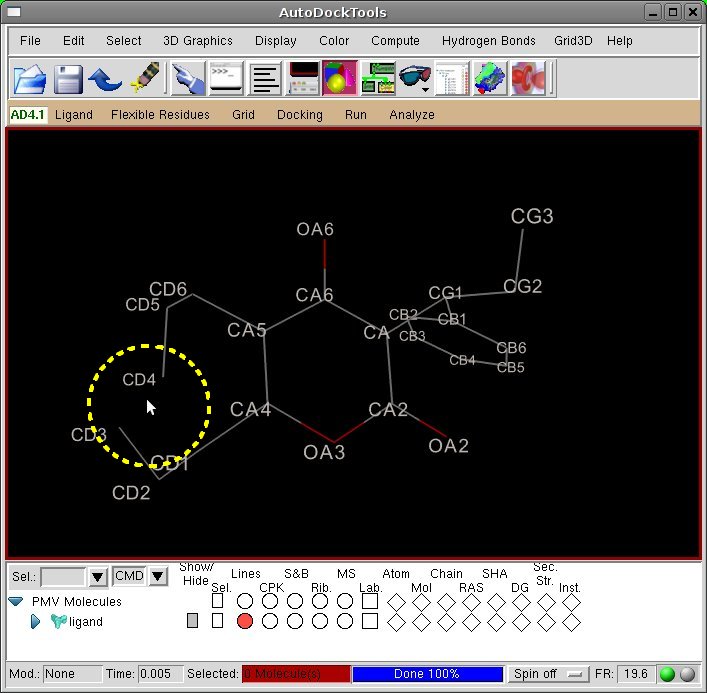
- The deletion of the
CD3-CD4 bond satisfied all the guidelines, leading to two short chains
(2 torsions) ending with non chiral C carbon atoms. Breaking the
CD1-CA4, for example, involves two different AutoDock atom types (C and
A, respectively). The deletion of the CD1-CD2 bond, on the other end,
would result in a single long flexible chain of 4 torsions. While being
not problematic for such a small ring, longer chains increase the
complexity of ring closure process in larger systems.
-Change the torsion angle of the ring chains; the
newly created chains will be modified to open up the ring and separate
the two edges atoms before adding hydrogens to the molecule:
[PMV Menu] Edit->Torsion angles
[Viewer] click on the four atoms defining the first torsion
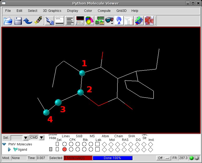 [Set Torsion Angles] modify the Set Angle value to pull apart the edge atoms, then click Done.
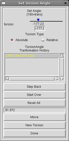
[Set Torsion Angles] click on New Torsion and repeat the torsion variation for the other chain.
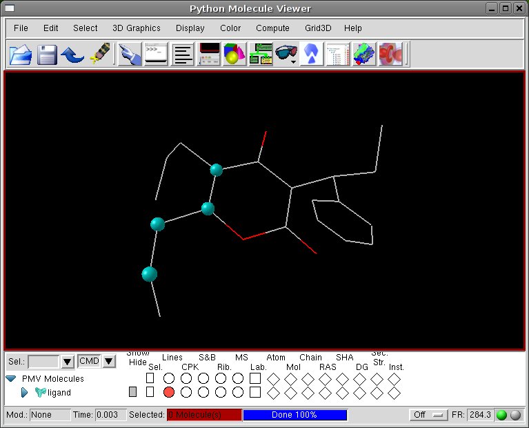
-The original ligand position from the X-ray structure is randomized to avoid any possible bias in the input conformation:
[PMV Buttons] Click on the DeJaVu icon 
[DeJaVu] (1) disable the option “mouse transforms apply to “root” object only”
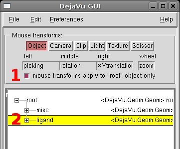
[DeJaVu] (2) select the ligand object “ligand”
[Viewer] Rotate and translate randomly the ligand
[PMV Menu] File->Save->Write PDB (check the “Save Transformed Coordinates” option, Filename: ligand.pdb)
-Clean up the session:
[PMV Menu] Edit->Delete->Delete All molecules, and press Continue
3. Generate the PDBQT file
-Process the input acyclic
structure following the standard AutoDock protocol by adding hydrogens
and selecting it for the PDBQT generation:
[PMV Menu] File->Read Molecule (ligand.pdb)
[PMV Menu] Edit->Hydrogens->Add (All Hydrogens, noBondOrder, yes)
[ADT Menu] Ligand->Input->Choose [or Open], select the ligand molecule name, then “Select Molecule for AutoDock4”
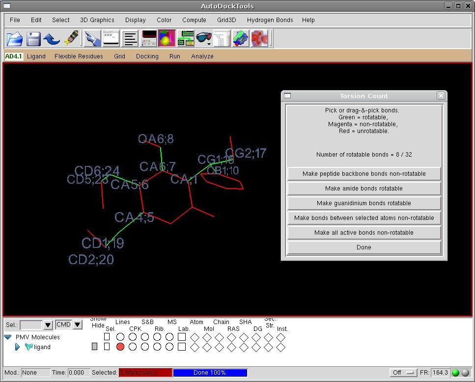
-Check the torsion tree:
[ADT Menu] Ligand->Torsion Tree->Choose torsion
- The torsion count window will now report the total number of rotatable bonds (8/32) activated for the ligand, including the chains formerly connected in the ring.
-If the rotatable bonds are correct, the structure can be saved and removed from the working session:
[ADT Menu] Ligand->Output->Save as PDBQT (ligand.pdbqt)
4. Specify the G atoms in the ligand
The carbon atoms previously connected will be manually renamed as "G".
-Make a copy of the original ligand file and name it as ligandG.pdbqt
-Open the file
ligandG.pdbqt in a text editor and locate the lines corresponding to
the edge atoms previously connected by the bond removed:
- HETATM 21 CD4 UIN B
100 -2.919 22.061
19.604 1.00 19.90 0.005 C
- [...]
- HETATM 24 CD3 UIN B
100 -3.821 22.402
20.791 1.00 19.60 0.005 C
-Modify the atom type definition by renaming the “C” atoms as “G” atoms in the last column:
- HETATM 21 CD4 UIN B
100 -2.919 22.061
19.604 1.00 19.90 0.005 G
- [...]
- HETATM 24 CD3 UIN B
100 -3.821 22.402
20.791 1.00 19.60 0.005 G
-Save the changes and close the text editor.
5. Prepare the protein and calculate grid maps
The special G atom does not need
specific maps being calculated.
For sake of ligand-protein interactions
a G atom is a C carbon tout-court, and in this way is parametrized in the
AutoDock energy parameters table. If a G map would be calculated with
AutoGrid, it will result in a file identical to the C map file. Therefore the C carbon maps are used for G atoms.
-Load the protein structure (“protein.pdb”) and add the hydrogens:
[PMV Menu] File->Read Molecule (protein.pdb)
[Dashboard] Click on the Sel. Button corresponding to the “protein” entry
[PMV Menu] Edit->Hydrogens->Add (All Hydrogens, noBondOrder, yes)
-Generate the PDBQT and set the grid maps:
[ADT Menu] Grid->Macromolecule->Choose->Select “protein”, then click on Select Molecule (press “OK”, and save it as protein.pdbqt)
[ADT Menu] Grid->Set Map Types->Choose Ligand->Select “ligand”, then click on Select Ligand
[ADT Menu] Grid->Grid box...
[Grid Options] Set
the number of points as 50, 50, 50 and center the box in the middle of
the dimer interface approximatively at coordinates: [0, 18, 20]
[Grid Options] File->Close saving current
[ADT menu] Grid->Output->Save GPF... (save it as protein.gpf)
-Run AutoGrid.
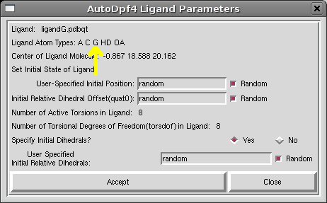
6. Generate the DPF and run the docking job
-Set the protein filename and define the atom type parameters (the G atom type is included automatically):
- [ADT Menu] Docking->Macromolecule->Set Rigid Filename->Select protein.pdbqt
- [ADT Menu] Docking->Ligand->Open...>Select ligandG.pdbqt (accept the default parameters clicking on “Accept”)
- [ADT Menu] Docking->Output->Lamarckian GA(4.2)Ligand-> Save it as ligandG_protein.dpf
-Edit the DPF file to include parameters for the ring closure.
The DPF file must be slightly
modified to set the special parametrization of the G atoms for driving
back together the edges of the ring during the docking and for tune the
search parameters accordingly to the increase of complexity. For more
complex searches, the ga_run and ga_num_evals values can also be increased. The file can be modified also with a text editor.
[ADT Menu] Docking->Edit DPF...
Edit the corresponding G atom map entry to point to the C maps:
Modify: “map protein.G.map” => “map protein.C.map”
Before
the "move" keyword, override the internal non-bonded parameter table
defining the pseudo-Lennard-Jones potential for the G-G interaction (req = 1.51 A, ε = 10 kcal/mol, n=12, m=2).
Add: “intnbp_r_eps 1.51 10.000000 12 2 G G“
The following parameters are changed only to increase the
Increase the GA population size from the default value to 350:
Modify: “ga_pop_size 50” => “ga_pop_size 350”
Increase the local search probability from the default value to 0.26 for helping the ring closure
Modify: “ls_search_freq 0.06” => “ls_search_freq 0.26”
Save the changes by clicking on "OK" and save the DPF
[ADT Menu] Docking->Output...->Lamarckian GA( 4.2)...
The final DPF should look like the following example (modified lines are in red and marked with “<===”):
autodock_parameter_version 4.1 # used by autodock to validate parameter set
outlev
1
# diagnostic output level
intelec
# calculate internal electrostatics
seed pid
time
# seeds for random generator
ligand_types A C G
HD
OA
# atoms types in
ligand
<===
fld
protein.maps.fld
# grid_data_file
map
protein.A.map
# atom-specific affinity map
map
protein.C.map
# atom-specific affinity map
map
protein.C.map
# C map used in place of G atom map <===
map
protein.HD.map
# atom-specific affinity map
map
protein.OA.map
# atom-specific affinity map
elecmap
protein.e.map
# electrostatics map
desolvmap protein.d.map # desolvation map
intnbp_r_eps 1.51 10.000000 12 2 G G # pseudo-LJ potential <===
move
ligandG.pdbqt
# small molecule
about -0.8665 18.5882 20.1623 # small molecule center
tran0
random
# initial coordinates/A or random
quat0
random
# initial quaternion
dihe0
random
# initial dihedrals (relative) or random
tstep
2.0
# translation step/A
qstep
50.0
# quaternion step/deg
dstep
50.0
# torsion step/deg
torsdof
8
# torsional degrees of freedom
rmstol
2.0
# cluster_tolerance/A
extnrg
1000.0
# external grid energy
e0max 0.0
10000
# max initial energy; max number of retries
ga_pop_size
350
# number of individuals in
population
<====
ga_num_evals
2500000
# maximum number of energy
evaluations
ga_num_generations 27000 # maximum number of generations
ga_elitism
1
# number of top individuals to survive to next generation
ga_mutation_rate
0.02
# rate of gene mutation
ga_crossover_rate
0.8
# rate of crossover
ga_window_size
10
#
ga_cauchy_alpha
0.0
# Alpha parameter of Cauchy distribution
ga_cauchy_beta
1.0
# Beta parameter Cauchy distribution
set_ga
# set the above parameters for GA or LGA
sw_max_its
300
# iterations of Solis & Wets local search
sw_max_succ
4
# consecutive successes before changing rho
sw_max_fail
4
# consecutive failures before changing rho
sw_rho
1.0
# size of local search space to sample
sw_lb_rho
0.01
# lower bound on rho
ls_search_freq
0.26
# probability of performing local search on individual <====
set_sw1
# set the above Solis & Wets parameters
unbound_model
bound
# state of unbound ligand
ga_run 10
# do this many hybrid GA-LS runs
analysis
# perform a ranked cluster analysis
Run AutoDock with the DPF:
autodock4 -p ligandG_protein.dpf -l ligandG_protein.dlg
7. Results analysis
The G atoms are included in the
internal energy parameters table AutoDock and are described by default
with carbon atoms parameters. For sake of ring closure, the
energy table is modified with the intnb_r_eps DPF keyword to define the pseudo-Lennard-Jones potential. The potential definition is logged in the DLG file:
|
      DPF> intnbp_r_eps  1.51 10.000042 12 2  G G #
pseudo-LJ
potential
Ring closure
distance potential found for atom type G :
Equilibrium distance = 1.51 Angstroms
Equilibrium potential = 10.000042 Kcal/mol
Pseudo-LJ coefficients = 12 - 2
Calculating
internal
non-bonded interaction energies for docking calculation;
Non-bonded
parameters for G-G interactions, used in internal energy
calculations:
281.0
27.4
E      =  -----------  -
-----------
G,G
12
2
r
r
|
The docking results can be compared with the X-ray conformation of the ligand:
-Clean up the session from all previous molecules and load the protein and the reference X-ray ligand:
[PMV Menu] Edit->Delete->Delete All molecules, and press Continue
[PMV Menu] File->Read Molecule (ligand_xray.pdb)
[PMV Menu] File->Read Molecule (protein.pdbqt)
-Load the DLG file and show the clustering results:
[PMV Menu] Edit->Delete->Delete All molecules, and press Continue
[ADT Menu] Analyze->Dockings->Open...->Select ligandG_protein.dlg
[ADT Menu]
Analyze->Clustering->Show...->Click on the cluster histogram
bars and browse the results with the conformations player.
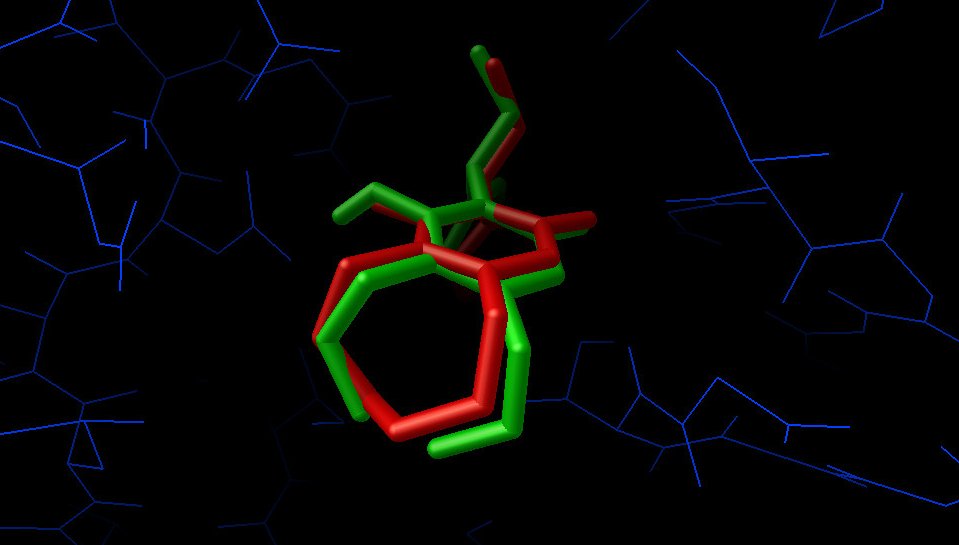
If the docking has been successful, the docked ligand overlapped with the experimental pose should look like this:
The red sticks shows the X-ray pose, while the green sticks are the docked result. The two G atoms are not be
represented as connected because they are not treated as carbon atoms by ADT.
Despite being very close to the crystal structure, the ring conformation and G-G bond distance are not . For this reason, a
molecular mechanics energy minimization is strongly adviced if any detailed
analysis and/or measurement is going to be performed.
8. Reference
If you are going to use this protocol, please cite the following paper:
All the images are generated with PMV.
9.Help
For any questions or help about the flexible rings or AutoDock usage, please use the forum or the mailing list.
Stefano Forli, TSRI, v0.1