Abstract
We describe a set of procedures and algorithms which have been developed to provide an efficient and reliable method for reconstructing a three dimensional density map from specimens with helical symmetry. These procedures build on the original MRC helical processing suite, with extensions principally developed using the SUPRIM image processing package. Actomyosin is used as a model specimen to demonstrate the utility of this repackaged and expanded set of routines. The time required to complete a 3-dimensional map has been reduced from several weeks using traditional manual techniques to a few days. The increased signal/noise provided has allowed for the extraction of additional layer lines not previously identified by manual techniques.
Introduction
Procedures for processing electron images of macromolecular structures with helical symmetry were originally developed at the MRC, Cambridge [1-4], and have been used successfully for many years for the determination of helical structures at moderate resolutions (9 - 30 Ĺ; for examples see [5-11]). The series of steps required to process electron images of helical structures are well documented and may be used consistently and reliably for the generation of 3-dimensional density maps. These procedures have traditionally relied heavily upon operator intervention to manually extract and manipulate data during the numerous processing steps. Such heavy demand on an operator's time is understandable, and perhaps even desirable, when processing a specimen of unknown selection rule for the first time as it requires the operator to pay careful attention to every step in the processing. The principal disadvantage of such a manual approach is that, by its time consuming nature, it limits the number of images which may reasonably be processed. It is not uncommon for an experienced operator using these procedures to spend several weeks processing the large number of images required to produce a single, averaged 3-D map at an appropriate resolution. While the resolution could be improved still further by increasing the number of images which contribute to the average [12], practical time considerations effectively limit what can reasonably be achieved. Furthermore, in situations where several independent 3-D maps are required for a thorough understanding of a structure, the time required of the operator for the image processing is an onerous burden. One final disadvantage is that the tedium of the task does not encourage repeating the processing either as a means of error checking or in order to measure the effects of alternative preparative or processing steps.
These disadvantages of the manual approach may be overcome through the judicious use of computational tools. At the most basic level, much of the operator input required when using the standard helical processing tools involves manually entering the results of one step as parameters to the next. This would be much more efficiently and rapidly handled by passing the parameters directly between the various computational steps without operator intervention. At a more complex level, there are a few critical steps where an intelligent decision must be made in order to extract the data. Examples of such steps include the straightening of the helical axis or the determination of layer line intercepts and the correct helical selection rule. Such steps require a computer algorithm which approximates the operator's decision-making processes.
In this paper we present procedures and algorithms which we have developed in order to provide a time efficient and reliable helical processing method. The approach we have taken bears many similarities to the approach of Morgan and DeRosier [12] in which they described a set of automated procedures which they used to extract data to 10Ĺ from the bacterial flagellar filament. The set of procedures presented here have been developed for Silicon Graphics workstations (or other workstations which utilize the SGI graphics language) as an extension of the original MRC helical processing suite [1-4], with extensions principally developed using the SUPRIM image processing package [13]. While many of the routines are copied or derived from these previously existing packages we have for the sake of simplicity and clarity assigned the name "PHOELIX" to this repackaged and expanded set of routines. The PHOELIX package is designed to run either in batch or interactive mode and in principal could proceed from a selected helical filament to the generation of a 3D density map without operator intervention. In practice the operator is provided with intermediate data which are used to evaluate the integrity of the results of each step. A number of automatic checks on these intermediate results will halt the process if any serious anomalies are detected. In addition, following the three critical steps where we have developed algorithms to emulate operator decisions, the results are presented to the operator and can be modified if necessary. When running in batch mode the processing runs to completion without any operator inspection. However a single command then presents the intermediate data to the operator in the same manner as in an interactive run. If the operator is required to modify the presented data in any way, all the subsequent steps may be repeated starting from the modified step.
Using actomyosin as a model specimen, the results obtained using the PHOELIX package are compared to our previously published actomyosin data which was obtained using standard manual image processing methods. We discuss these results in terms of both the time required for the processing and the quality of the resulting data. We also discuss the applicability of these procedures to specimens other than actomyosin.
Description of the PHOELIX Package
Overview
The overall design of the software adheres to a very modular structure in which data is sequentially passed along a series of individual processing steps. These steps are controlled by a UNIX shell script which may be readily edited to modify, reorder, add or delete steps as required by the operator. The individual software modules which operate on the data have been largely drawn, or derived from, two software packages, SUPRIM [13] and programs written originally at the MRC, Cambridge [1-4]. In choosing to use the SUPRIM software package as a basis for PHOELIX we were influenced by the very modular approach to the problems of image processing taken by this package and also its high level of organization and documentation. This has made the process of adding new modules and modifying existing ones very straightforward. The MRC helical software routines were used to perform the Fourier-Bessel reconstruction because these routines are very widely used and accepted. The overall modular design of the current package allows for the incorporation of new or modified MRC code in a straightforward manner. Libraries used for the MRC routines compatible with the UNIX operating system were generously provided by Michael Schmid and Wah Chiu of Baylor College of Medicine. Other routines were ported to or rewritten for the UNIX operating system as required.
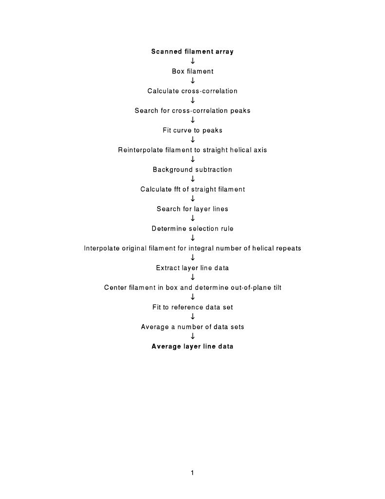
An overview of the semi-automated helical reconstruction procedure is represented schematically in figure 1. Those steps which have been written specifically for PHOELIX will be described in some detail in the following paragraphs. For those steps which have been drawn from the MRC helical processing suite it is suggested that the original publications be used as a reference [1-4]. We will use actin decorated with myosin II subfragment 1 (acto-S1) as a model specimen throughout this discussion. An extensive appendix to this document containing additional documentation on all software modules used in the PHOELIX package is omitted here for brevity. It is available as part of the PHOELIX distribution.
Straightening the filament
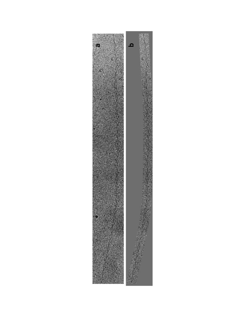
Cryoelectron images of acto-S1 were recorded under low dose conditions and selected filaments converted into digital density arrays as described previously [8]. A typical digitized array is shown in figure 2a. In order to isolate the filament from surrounding noise, other filaments, etc., a box is constructed by having the user interactively specify a few points tracking the axis of the filament of interest. Using these specified points a curve is fitted to the axis and the filament is isolated by boxing off a region of a given width around the curve ("snake" boxing). This is illustrated in figure 2b.
Filaments selected for processing often exhibit a slight curvature along their length. While it is possible to identify short segments of a filament which are essentially straight, such regions are not generally more than a few helical repeats in length. Processing much longer straight filaments increases signal/noise, thus making it easier to index the helical diffraction pattern and extract layer line data. Additionally, longer filaments reduce the number of filaments which must be densitometered, processed, and reconstructed and so also reduce the overall time and effort necessary to obtain a final 3D density map. Computational straightening of a curved filament [14] is now a well established technique and is performed as a matter of routine as an initial step during processing. The straightening procedure begins by calculating a Fourier-space cross correlation map between a template and the curved filament. The template can consist of either a short segment of the filament under consideration or a short section of an average structure calculated from an initial 3-D map (inset in figure 3a). The cross correlation map thus calculated will have a series of maxima along the helical axis. We have found that identification of these peaks is often made easier if the digitized image is first low pass filtered prior to calculating the cross correlation map. This step is at the discretion of the operator and the filtered image is discarded once it has been used to help define the helical axis of the original image.
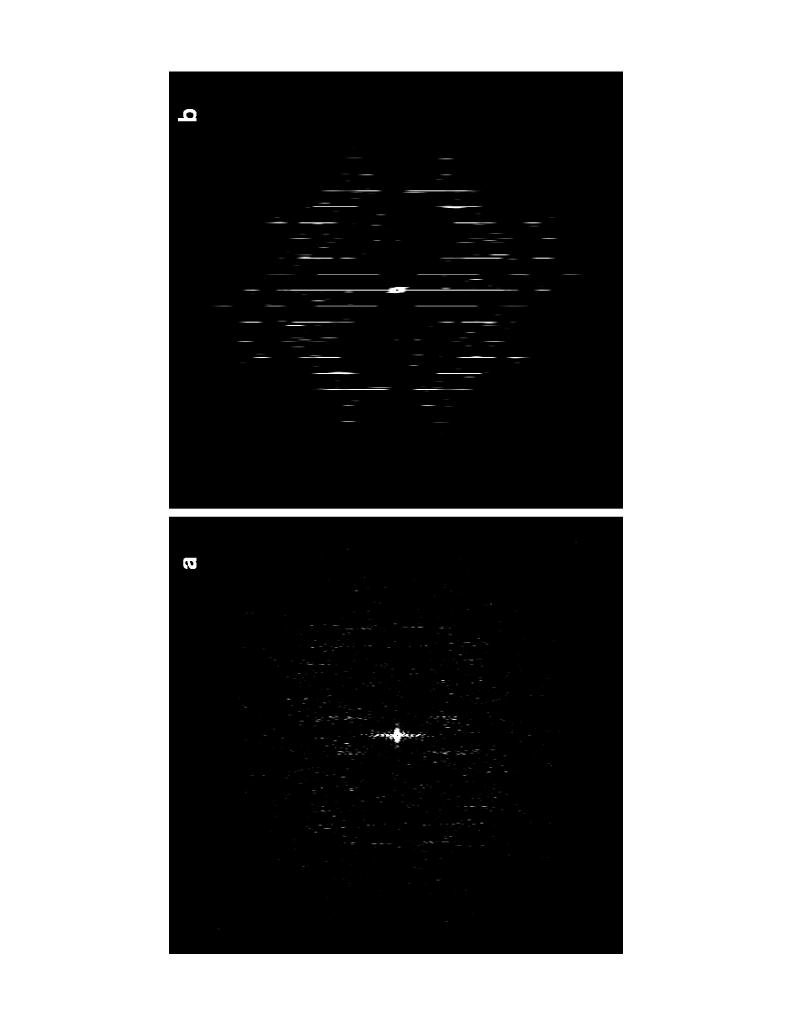
Precise peak locations and values are determined using a parabolic fit in a 3x3 neighborhood around the highest values in the cross correlation map. The number of peaks expected to lie on the filament axis is estimated by calculating the number of times the length of the template divides into the total length of the filament. As a number of peaks will be identified which are not precisely on the filament axis, the total number of peaks examined is this expected value times some multiplier, in this case 3 (figure 3a). The set of identified peaks are then passed along to a routine which is designed to identify and eliminate the spurious peaks. It does so by starting with the highest peak (assuming that this highest peak is on the helical axis) and then working along the helical axis in both directions rejecting peaks that are outside of certain defined error limits. These error limits are defined to reject peaks which are either too close together along the helical axis or which show too rapid a change perpendicular to the axis. These criteria are highly effective in identifying an axis which is free of spurious points and work perfectly for about 90-100% of the filament length (figure 3b). The method fails occasionally when a peak passes all of the error requirements but is still off the axis of the filament. Usually this peak can be simply deleted during the interactive examination of the selected axis, resulting in a curve which is smooth and continuous along the length of the filament. The curve which is fitted to the axis points may be selected to be either a cubic spline or a low order polynomial. A straightened image of the curved filament is calculated by interpolating the filament along lines perpendicular to the fitted curve. The power spectra of a filament before and after straightening are shown in figure 4.
Background subtraction
The straightened filaments can be greater than 1 micron in length. For cryoelectron micrographs it is not unusual for there to be significant variation in the thickness of the ice layer over this distance, resulting in a non uniform background over the image. This non-uniformity in turn introduces low frequency artifacts into the Fourier transform which may affect the amplitudes and phases of the low order layer lines extracted from these transforms. This problem may be reduced if the background variations are subtracted from the image prior to calculating the transform. This is achieved by extracting the first and last rows of the straightened filament, fitting a polynomial curve to the intensities along these two rows, calculating an interpolated surface defined by these two curves, and subtracting this from the original image. During this procedure the image is also floated to a mean value of zero.
Identification of layer lines
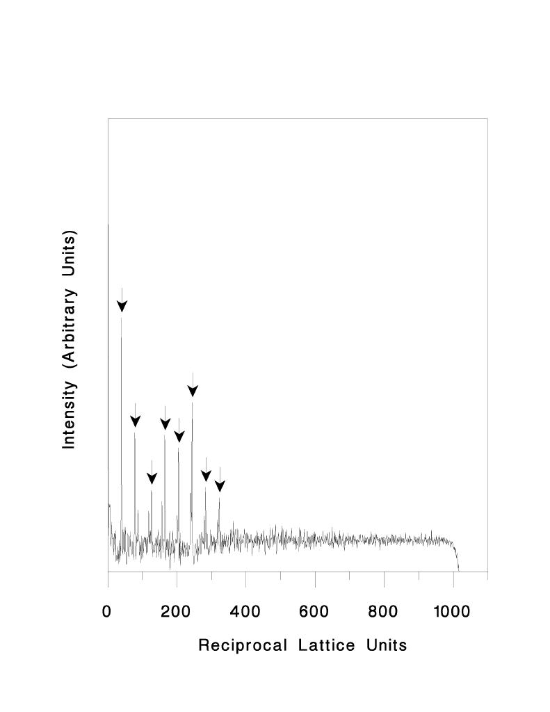
In order to extract the layer lines from the transform they are first located in the following manner. A region around the meridian of the power spectrum which contains strong amplitudes is excised from the transform and the integrated intensities perpendicular to the meridian are plotted versus transform pixel number. The background of this curve is removed by calculating a very low pass filtered image of the curve and subtracting this from the original. The result is illustrated in figure 5. A peak searching algorithm is then used to search for a number of peaks at set intervals along the curve which are more than a given number of standard deviations above the background. The interval used is the approximate location of the first layer line, determined from the user-provided crossover length of the helix. The peaks which are identified in this way are noted in figure 5.
Determination of the correct selection rule
The layer line positions which are identified in the peak search are assigned layer line numbers and Bessel orders according to a list of possible selection rules provided by the operator (table 1). A linear regression algorithm is used to determine the selection rule which gives the best fit to a straight line for layer line position versus layer line number. If none of the provided selection rules give a good fit (c2 < 1), a warning message is sent to the operator. Once the best selection rule has been determined the filament is reboxed so as to contain an integral number of helical repeats which are exactly enclosed in an array which is 2n in length. This is done so that the computed layer lines will lie exactly on the transform sampling raster. The reboxing is performed by reinterpolating the image from the original curved filament, thus creating an interpolated and straightened image in a single step. The selection rule of this new straightened image is checked for consistency with the selection rule determined during the initial straightening. Finally, this image is background corrected and floated to a mean density of zero as described above (figure 3c).
Extracting the layer line data
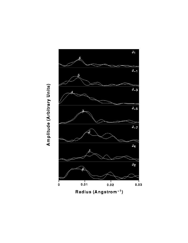
The layer line spacing for the final straightened filament is determined from the intercepts of certain specified strong layer lines. For the data shown here the J2 and J- 1 Bessel orders are used, and the spacing is determined by summing the layer line intercepts and dividing by the sum of the layer line numbers (e.g. for a 13/6 selection rule, if the intercept of layer line 1 was at 10 reciprocal lattice units (rlu), and the intercept of layer line 6 was 60 rlu, the average spacing would be (10+60) / (1+6) = 10 rlu). This average spacing is used to predict layer line intercepts out to some defined resolution. For those layer line intercepts which were located as peaks in the 1-D array during the determination of the selection rule, the located intercept rather than the predicted intercept is used. If this located intercept differs by more than 1 rlu from the predicted intercept, a warning message is sent to the operator. In interactive mode the operator is presented with a power spectrum of this questionable region of the transform and asked to decide whether to use the predicted or located intercept. Alternatively, an intercept of the operator's choosing may be selected. In batch mode the located intercept is used and the operator may decide to accept or correct this value at a later time. The intercepts are written into a parameter deck required by the MRC helical program suite and used to extract layer lines from an MRC format transform file. Further processing, including correction for out-of-plane tilt, centering in the transform box, fitting to a reference data set and averaging was performed essentially as previously described [8]. Correction for tilt and centering require the operator to specify amplitude peaks on certain strong layer lines which approximately match across the meridian. These peaks are determined computationally by identifying the amplitude maximum in the vector average of the near and far side of each layer line. In interactive mode the amplitude peaks selected in this way are presented graphically to the operator (figure 6) and may be edited.
Use of the PHOELIX package
In practice an operator would begin a new reconstruction by editing a number of values in a global parameter file. These would include the list of possible selection rules, approximate crossover distance, Bessel orders of the strongest layer lines and a number of other critical parameters which control the procedures and software modules. The parameter file which was used for all of the acto-S1 filaments used as examples in this paper is shown in section 3 of the appendix. While some of the controlling parameters (e.g. selection rule, strong Bessel orders, etc.) can be measured directly from the data, others (straightening parameters, radius of low pass filter, etc.) might need to be empirically determined. The entire process runs rapidly enough (~ 5 minutes per filament) so that a large number of parameter values may be tested in a relatively short time. Once a set of parameters has been determined to work for a given helical filament it should be possible to use them for all further processing of this structure.
The filament must be in SUPRIM format, boxed (using a rectangular or snake box) and oriented with its long axis parallel to the x axis. The template may be either a small piece of the original filament or a model structure determined from a previously calculated map. Once the parameter file has been set up and the filament and template have been selected, the operator begins a reconstruction by starting the main controlling script using the command:
"s_phoelix [filament name] [template] | tee > [output file]"
If the processing is running in interactive mode the information written to the output file will also be echoed to the screen. This information consists of terse comments detailing the actions taken by each script which is called and relevant data pertaining to the results of these actions. These data include the list of layer line intercepts for the strong Bessel orders which are used to determine the selection rule, the chosen selection rule and the c2 value representing the goodness of fit to this selection rule, the location of each strong layer line intercept in relation to its predicted value, tilt/shift search results, and results of the fit to a reference data set. In addition, the operator is presented with a number of graphical displays including the location of the cross correlation peak values used to straighten the filament, the collapsed power spectrum, the final reinterpolated filament and its power spectrum, and layer line data indicating the radial positions of the peaks used in the tilt/shift search. The operator is also prompted for input at the following points: 1) approval or correction of the cross correlation points used for straightening the filament; 2) choice of layer line intercept when the determined intercept differs by more than one pixel from the predicted value; and 3) approval or correction of the amplitude peaks chosen for out-of-plane tilt and axis centering correction.
If these procedures are run in batch mode, the graphical output may be viewed at a later stage to assess the success of the processing steps. During this examination any of the parameters requiring operator approval may be edited and the processing restarted from that point.
Results
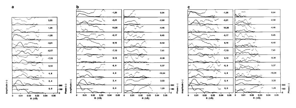
The procedures presented here were initially tested by processing cryoelectron images of actin decorated with S1 containing the alkali 2 light chain (acto-S1(A2)). The final layer lines are an average of 14 individual data sets (near- and far-side layer lines from 7 filament images). For each filament, the selection rule was 54,25 (the majority of our decorated actin filaments fit best to this selection rule). Those few filaments which did not conform to this selection rule or which fit only poorly were not included in the average. Approximately half of the filaments we have processed required intervention by the operator during the straightening step or the step in which peaks are selected to use for correcting out-of-plane tilt and axis centering of the filament. These interventions were typically as simple as deleting a single automatically-determined point. The average length of each filament was approximately 1.15µm, representing 8 repeats of the 54/25 helix. The final average layer line data, representing a total of 3024 individual acto-S1(A2) subunits, are shown in figure 7b. Data obtained by manually processing a large number of short, naturally straight regions of filament are shown for comparison in figure 7a. By manual processing, a total of 10 layer lines were identified, extending to a resolution of 45 Ĺ axially and 35 Ĺ radially. The increased signal/noise ratio provided by the long, straightened filaments enabled us to define the selection rule better and to identify a total of 22 layer lines extending to ~27 Ĺ in all directions. In addition to those layer lines beyond the J3 which had previously not been identified, we were able to extract a number of layer lines at low resolution (e.g. J-9) which had been missed previously. Although the amplitudes of the higher resolution layer lines (layer lines 34-54) are weak, the data are reliable as phases across the amplitude peaks are reproducible in data representing the same structure calculated from independent populations of filaments (data not shown).
One consequence of processing long filaments using these procedures is an attenuation of layer line amplitudes at increasing meridional spacing. For example, the J2 layer lines in the current data set and in the previously published data set have approximately equal amplitudes (see figure 7 a and b). In contrast, the amplitudes on the J-1 layer line in the current data set have been reduced by approximately 25% relative to the earlier data set. The observed attenuation is likely a result of small variations in pitch along the length of these very long filaments [17-20]. Indeed, the pitch probably varies from monomer to monomer rather than from repeat to repeat. As a result, layer lines which should be a single pixel in width are blurred somewhat onto surrounding pixels. This attenuation of amplitudes may be reduced if the long straightened filaments are broken into shorter segments, each containing an integral number of repeats, and processed separately (data not shown). This does, however, increase the noise in transforms from individual filaments, which makes the determination of the selection rule more difficult. It also increases the number of computations, and therefore the time required, to complete a map. As a simpler correction, amplitudes are extracted by axial integration across several pixels in the transform, centered on the calculated layer line position. The amplitude component is determined from a vector addition across three pixels centered on the layer line and the phase component taken from the center pixel, where the amplitude is highest and the phase best defined. The resulting average layer lines are presented in figure 7c. A comparison of the layer lines in this new data set to that presented in figure 7b, shows that while the amplitude of the J2 remains approximately unchanged the J-1 amplitude is no longer attenuated relative to the previously published data.
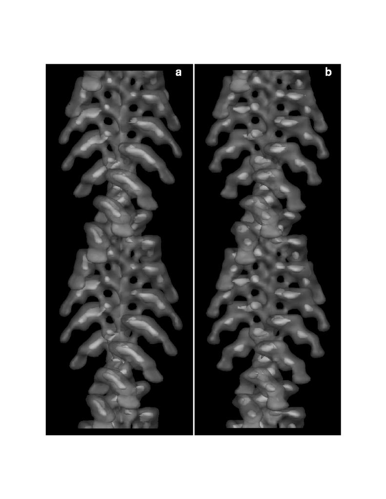
Three dimensional maps were calculated by Fourier-Bessel inversion of the layer line data in figures 7 a and c. The maps are surfaced at a contour level which encloses approximately 100% of the expected mass of the structures and these surfaces are displayed in figure 8. All of the features which were present in the earlier map are also present in the new map. However, as a result of the additional layer lines identified by processing long straightened filaments, the surface envelope of the structure is more detailed and contours at 10% of the expected mass (the internal contours in figure 8) show that peak density which was an elongated smear has now been resolved into two sharp density peaks .
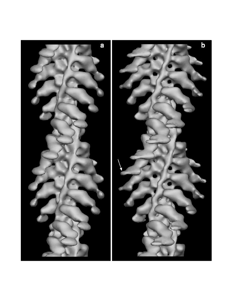
The processing of acto-S1 demonstrated the utility of these procedures and allowed us to gain experience in using them. To estimate the length of time required for an experienced user to complete a new reconstruction we next analyzed images of a related structure: the thin filament (actin + tropomyosin + troponin) decorated with S1 containing both the alkali and DTNB light chains (TFS1). The final layer line data are an average of 12 data sets (6 filaments, 1512 molecules; not shown). Beginning with scanned density arrays, a complete reconstruction (i.e. collection of final average layer lines and calculation of a 3-D density map) was performed in a single day. A statistical comparison to the acto-S1(A2) map discussed above required a second day of computing. This compares very favorably to the approximately 3-4 weeks required to calculate an earlier map of the same structure using traditional image processing techniques [16]. This earlier map was calculated from a large number of short, naturally straight filaments, for which a 13,6 helical selection rule was assumed. The earlier average was calculated from 1339 TFS1 molecules, compared to 1512 molecules in the new map. In a difference map calculated between the earlier TFS1 map and a map lacking the DTNB light chain there was no statistically significant density identifiable as the light chain (figure 9a). In contrast, a comparison of maps determined by processing long filaments using PHOELIX show additional highly significant density at high radius which we ascribe to this light chain (figure 9b). A full account of these data will be published elsewhere.
Conclusions and Future Prospects
We have developed a semi-automated set of procedures for the processing of helical filaments and demonstrated its utility by applying it to actomyosin. These procedures dramatically reduce the time taken to complete a map and result in a three dimensional data set with a resolution better than that achieved using manual methods. The package in its current form has been optimized for the processing of actomyosin filaments but has also been successfully applied to undecorated actin. The modular design should readily accommodate any modifications necessary to apply these procedures to other helical structures.
One goal in developing this package was simply to streamline the helical reconstruction procedures so that they might be performed quickly and routinely. This goal has been met and it is now possible to complete a 3-D map in a day or two, a process that would have taken several weeks previously. As a further advantage of the increased efficiency of the reconstruction process we are able to experiment with the parameters and individual processing steps in order to optimize conditions for our particular data set. The procedures can also be easily and quickly repeated by a number of different operators in order to explore the effects of subjective bias on the final outcome.
A second goal for these procedures was to increase the length of the filaments as well as the total number of molecules contributing to the final average layer line data in a given map. The resulting overall increase in signal/noise has allowed for more precision in the identification of layer lines and in the determination of the helical selection rule as compared to our previous maps. We have been able to extend the nominal axial resolution of our maps from 45Ĺ to 27Ĺ and to collect previously unidentified layer lines at low resolution. These improvements in the data have enabled us to locate the DTNB light chain in actoS1. The ability to identify an additional light chain in maps calculated using PHOELIX as opposed to maps calculated using manual techniques was particularly significant. The two maps were calculated from averages containing approximately equal numbers of molecules, indicating that the increase in precision of the image processing steps provides much of the improvement seen in the final data.
A further extension of the resolution is probably limited by remaining disorder in the specimen and by difficulties inherent in collecting electron images of frozen specimens, e.g. inelastic scattering, specimen movement, and charging [21]. These limitations may be thought of as analogous to those caused by thermal motion in X-ray crystallographic studies, albeit on a larger scale. By analogy then, one can describe these limitations as contributing to a "temperature factor" which describes a reduction in scattering power of a molecule as a result of disorder and imaging difficulties. Previous work has described limits in structure factor amplitudes at high resolution resulting from temperature factors and noise, using 2-D crystals of bacteriorhodopsin as a model [22]. The authors describe a strong attenuation of amplitudes which becomes progressively worse as the temperature factor is increased. Additionally, as the signal/noise decreases at high resolution, the extraction of accurate phase information becomes problematic. With a crystalline specimen such as bacteriorhodopsin, such difficulties become very important at high resolution and may be overcome by combining amplitudes obtained from electron diffraction patterns with phases from the electron images. For helical structures which are both very weak diffractors [12] and, in the case of actomyosin, much more poorly ordered than the crystals, these temperature factor effects become significant at the moderate resolution described here.
Possible sources of disorder in the actomyosin filaments used in this study include errors in axis straightening, variability in helical pitch, and variations in out-of-plane tilt along the filament. Initially, the accuracy of the straightening algorithm could be perhaps improved. For example, peaks in the cross correlation map can be sharpened up considerably by orienting the template to more closely match the local orientation of small sections along the filament. Additional improvement may be obtained by the incorporation of iterative techniques similar to real-space methods described for 2-D crystals (whereby a projection of the calculated 3-D map is used as a reference to re- straighten and re-process the images) [23] or correlation functions which emphasize high resolution features in images [24]. It should be noted that the modular nature of PHOELIX makes addition of modules with new features very convenient. Errors due to noise in the image are however likely to remain a problem, particularly for ice embedded specimens, where the contrast is low.
Variability in helical pitch [17-20] is a much larger source of remaining disorder in these filaments, as was demonstrated by the attenuation of layer line amplitudes seen in figure 7. As noted, it was possible to improve the data by breaking the filament into shorter and shorter lengths, though this sacrifices signal/noise and significantly increases computational requirements. The simpler correction of collecting data by integration across a number of pixels in the transform appears to provide an approximately equivalent improvement in the data, albeit at the expense of increased noise on weak layer lines. Further improvements might be achieved by explicitly measuring and taking into account the instantaneous pitch along each filament. This approach has been successfully applied in the analysis of sickle hemoglobin filaments [25], and could be used for actomyosin now that the high resolution x-ray crystal structures of both actin [26,27] and the myosin head [28,29] are available. Similarly, local variations in out-of-plane tilt along the filament can be measured [12], and while algorithms for their correction have yet to be described, techniques akin to those applied for the correction of variable pitch should be applicable.
A further increase in the signal-to-noise ratio of high resolution layer lines might be achieved through the use of a layer line "sniffer" algorithm as described by DeRosier [30]. In this algorithm an initial set of average layer lines is calculated by extracting and averaging data from individual filaments for which the predicted positions of high resolution layer lines has been determined from the selection rule. As a result of disorder in the filaments the actual layer line position might differ from the predicted layer line position, particularly at increasing resolution. The sniffer algorithm thus calculates a phase residual between each layer line in the average data set and each of a set of layer lines centered around the predicted layer line position in the individual filament. The layer lines corresponding to the lowest phase residual are then used to compute a second average and the process is iterated until no further improvement is achieved.
Finally, while these corrections may help to compensate for specimen disorder, they do not address those difficulties inherent in recording electron images. It may be possible to attempt a correction for these difficulties similar to that described by Schertler, Villa and Henderson [31]. In this study the attenuation of amplitudes computed from electron images of rhodopsin was determined by comparison to electron diffraction patterns obtained from bacteriorhodopsin. This amplitude correction relies on the similarity between rhodopsin and bacteriorhodopsin and would not be directly applicable to actomyosin. It might be possible, however, to obtain a similar correction by computing a diffraction pattern from a "model" actomyosin filament based on the x-ray crystallographic map of actin and myosin molecules. Comparison of the theoretical layer line amplitudes to our calculated average amplitudes would provide an equivalent temperature factor correction.
The current implementation of the PHOELIX package is available on request. Send email to bcarr@uiuc.edu or mike@scripps.edu.
Acknowledgments:
We thank Wah Chiu and Mike Schmid (Baylor College of Medicine) for generously providing UNIX-compatible versions of the MRC image libraries. This work was supported by grant AR39155 (to R.A.M.) from the National Institutes of Health. R.A.M. is an Established Investigator of the American Heart Association.
Figure 1. Schematic diagram of the PHOELIX helical processing package. Those procedures which were developed specifically as part of PHOELIX are discussed in the text. For those procedures taken from the MRC helical image processing package additional documentation is available in the original publications [1-4] and with the PHOELIX distribution.
Figure 2. Boxing of the densitometered filament image. Images of filaments were converted to computer density arrays using a Perkin Elmer 1010G densitometer operating with 25 µm spot and step sizes (7.14 Ĺ at the image). A typical filament which has been boxed rectangularly is shown in panel a and an image which has been "snake" boxed is shown in panel b.
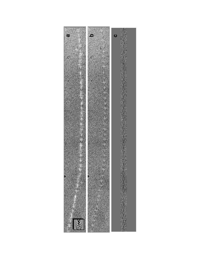
Figure 3. Intermediate stages in the straightening process. The template used for cross correlation (inset in panel a) is a projection of one crossover (360 Ĺ) of acto-S1, shown here for clarity at twice the scale of the other panels in the figure. Peak values from the cross correlation map, calculated as described in the text, are displayed overlying the filament (a). Beginning with the highest peak, neighboring peaks are compared. A peak is discarded if, compared to the preceding peak, it is closer than 40 pixels in x, or diverges further than 12 pixels in y and has a slope (i.e. *y/*x) greater than 0.3. The remaining peaks (b) are used to define the filament axis. A cubic spline is fit to these points, and the curve is used to map the filament onto a linear helical axis. This straightened filament image is then background corrected and used for determination of the selection rule. Using the chosen selection rule, the original filament image is reinterpolated and restraightened such that an integral number of helical repeats precisely fills a box suitable for Fourier transformation (c).
Figure 4. Power spectra of an unstraightened (figure 1b) and straightened filament (figure 2c) are shown in panels a and b, respectively.
Figure 5. Identification of layer line intercepts. The power spectrum in figure 3b is collapsed to a 1-dimensional array and corrected for background as described in the text. Peaks which are more than 3 standard deviations above the background and which are located at the predicted layer line spacings (within a given range) are indicated by arrows.
Figure 6. Amplitude peaks used for correction of out-of-plane tilt and centering of the filament in the transform box. Near and far side amplitudes of those layer lines identified as "strong" are displayed together. Note that on the workstation screen the near and far side data are displayed in different colors for clarity. The maximum value in the vector average of each layer line is computed and marked with a "+". These amplitudes and phases are extracted for tilt and shift determination.
Figure 7. Final S1(A2) layer line averages. (a) The 10 layer lines obtained by manual processing of short, straight regions of actomyosin [16]. (b) The 22 layer lines obtained using PHOELIX. (c) As in b, except that amplitudes are the vector sum of three pixels centered on the layer line intercept. Amplitudes on layer lines 34-54 have been scaled 3x.
Figure 8. Surface views of acto-S1(A2). Three-Dimensional maps were calculated from our previously published data (a) and from data obtained from straightened filaments (b) by Fourier-Bessel inversion of the layer line data in figures 6a and c, respectively. The surface enclosing ~100% of the expected mass of acto-S1(A2) is displayed here transparently to allow viewing of an internal solid contour representing 10% of the expected total mass of the structure. Surfaces are visualized using the program SYNU [15]. It is the map displayed in panel b which was used to model the atomic structures of actin and S1 into a filament [27].
Figure 9. Surface views of the decorated thin filament. The surfaces have been calculated from our previously published data [16] (a) and from data obtained from straightened filaments (b). By calculating difference maps between maps containing and lacking the DTNB light chain, the additional mass at high radius in panel b (arrow) has been identified as representing the DTNB light chain domain.
Table 1Layer line numbers and Bessel orders for various helical selection rules.
Bessel Order Layer Line Number (selection rule)
(13/6) (28/13) (41/19) (54/25)
J0 0 0 0 0
J2 1 2 3 4
J4 2 4 6 8
J-9 2 5 7 9
J6 3 6 9 12
J-7 3 7 10 13
J8 4 8 12 16
J-5 4 9 13 17
J10 5 10 15 20
J-3 5 11 16 21
J-1 6 13 19 25
J1 7 15 22 29
J3 8 17 25 33
J-10 8 18 26 34
J5 9 19 28 37
J-8 9 20 29 38
J7 10 21 31 41
J-6 10 22 32 42
J9 11 23 34 45
J-4 11 24 35 46
J-2 12 26 38 50
J0 13 28 41 54
References
[1] Moore, P.B., H.E. Huxley, and D.J. DeRosier. J. Mol. Biol. 50 (1970) 279-295
[2] DeRosier, D.J. and P.B. Moore. J. Mol. Biol. 52 (1970) 355-369
[3] Wakabayashi, T. , H.E. Huxley, L.A. Amos and A. Klug. J. Mol. Biol. 93 (1975) 477-497
[4] Amos, L.A. and A. Klug. J. Mol. Biol. 99 (1975) 51-73
[5] Taylor, K.A. and L.A. Amos. J. Mol. Biol. 147 (1981) 297-324
[6] Vibert, P. and R. Craig. J. Mol. Biol. 157 (1982) 299-319
[7] Toyoshima, C. and T. Wakabayashi. J. Biochem. 97 (1985) 219- 243
[8] Milligan, R.A. and P.F Flicker. J. Cell Biol. 105 (1987) 29-39
[9] Unwin N. J. Mol. Biol. 229 (1993) 1101-24
[10] Schmid, M.F., J.M. Agris, J. Jakana, et al. J. Cell Biol. 124 (1994) 341-350
[11] McGough, A., M. Way, DeRosier, D. J. Cell Biol. 126 (1994) 433- 443
[12] Morgan, D.G. and D. DeRosier. Ultramicroscopy 46 (1992) 263- 285
[13] Stoops, J.K., Schroeter, J.P., Bretatudiere, J.P., Olson, N.H., Baker, T.S., and Strickland, D.K. J. Struct. Biol. 106 (1991) 172-178.
[14] Egelman E.H. Ultramicroscopy 19 (1986) 367-373
[15] Hessler, D., Young, S.J., Carragher, B.O., Martone, M., Hinshaw, J.E., Milligan, R.A., Masliah, E., Whittaker, M., Lamont, S. and Ellisman, M.H. Microscopy 22(1) (1992) 73-82.
[16] Milligan, R.A., M. Whittaker and D. Safer. Nature 348 (1990) 217- 221
[17] Hanson, J. Nature 213 (1967) 353-356
[18] Egelman, E.H., and D.J. DeRosier. Acta Crystallogr. A. 38 (1982) 796-799
[19] Aebi, U., R. Millonig, H. Salvo, et al. Ann. N.Y. Acad. Sci. 483 (1986) 100-119
[20] Stokes, D.L. and D.J. DeRosier. J Cell Biol. 104 (1987) 1005- 1017
[21] Henderson, R. Ultramicroscopy 46 (1992) 1-18
[22] Glaesar, R.M. and K.H. Downing. Ultramicroscopy 47 (1992) 256- 265
[23] Crepeau, R.H. and E.K. Fram. Ultramicroscopy 6 (1981) 7-18
[24] Schatz, M. and M. van Heel. Ultramicroscopy 45 (1992) 15-22
[25] Bluemke, D.A., B. Carragher, and R. Josephs. Ultramicroscopy 26 (1988) 255-270
[26] Kabsch, W., H.G. Mannherz, Suck, D., et al. Nature 347 (1990) 37- 44
[27] Holmes, K.C., D. Popp, W. Gebhard, et al. Nature 347 (1990) 44- 49
[28] Rayment, I., W.R. Rypniewski, K. Schmidt-Base, et al. Science 261 (1990) 50-58
[29] Rayment, I., H.M. Holden, M. Whittaker, et al. Science 261 (1993) 58-65
[30] Morgan, D.G. and D. DeRosier. Biophys. J. 64 (1993) a243
[31] Schertler, G.F.X., C. Villa, and R. Henderson. Nature 362 (1993) 770-772